Solving Gymnasium's Lunar Lander with Deep Q Learning (DQN)

Introduction

Reinforcement learning is an interdisciplinary area of machine learning that has gained popularity in the last decade due to its recent accomplishments in games like Go and real-world applications like self-driving cars. This growth has also coincided with the rapid advancements in modern GPUs and the evolution of machine learning techniques. We have reached a stage where machines can easily outperform humans in computer games. Deep Q-Network (DQN) is a new reinforcement learning algorithm showing great promise in handling video games such as Atari due to their high dimensionality and need for long-term planning. This tutorial will explain how DQN works and demonstrate its effectiveness in beating Gymnasium's Lunar Lander, previously managed by OpenAI.

What is Reinforcement Learning?

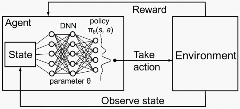
Deep Reinforcement Learning: Value Functions, DQN, Actor-Critic method, Back-propagation through stochastic functions | by Vishnu Vijayan PV | Medium

Reinforcement learning involves an agent making decisions by performing actions in an environment to maximize cumulative rewards. Key components of RL include:

Agent: The decision-maker interacting with the environment.
Environment: The external system with which the agent interacts.
State (S): The current situation or configuration of the environment.
Action (A): The possible moves or decisions the agent can make.
Reward (R): Feedback from the environment indicating the quality of an action.
Policy (π): A strategy mapping states to actions that define the agent's behavior.
Value Function (V): Estimates the expected cumulative reward from a given state.
Q-Function (Q): Estimates the expected cumulative reward of taking a particular action in a given state.

How Reinforcement Learning Works

Initialization: The agent starts with no or minimal knowledge about the environment.
Interaction: The agent interacts with the environment by taking actions based on its policy.
Feedback: The environment responds to each action with a new state and a reward.
Learning: The agent updates its policy and/or value functions based on received rewards to improve future decisions.

Key Concepts

Exploration vs. Exploitation: Balancing the exploration of new actions and the exploitation of known high-reward actions.
Discount Factor (γ): Determines the importance of future rewards relative to immediate rewards.
Bellman Equation: Describes the relationship between a state's value and its successor states' values.

The Bellman Equation

The Bellman equation is fundamental in reinforcement learning, providing a recursive decomposition of the value function. It relates the value of a state to the values of subsequent states. The Bellman equation for the Q-function is given by:

$${{Q(s, a)=r+γ \max_{a'} Q(s', a')}}$$

Here:

${{Q(s, a)}}$ is the Q-value for taking action aaa in state sss.
${{r}}$ is the reward received after taking action aaa.
${{\gamma}}$ is the discount factor, determining the importance of future rewards.
${{\max_{a'} Q(s', a')}}$ is the maximum Q-value for the next state ${{s'}}$ over all possible actions ${{a'}}$.

Temporal Difference Learning

Temporal difference (TD) learning is a key approach in RL, combining ideas from dynamic programming and Monte Carlo methods. It updates the value functions based on the difference (or temporal difference) between the predicted value and the actual received reward plus the discounted value of the next state.

The update rule for Q-learning, a type of TD learning, is:

$${{Q(s, a) \leftarrow Q(s, a) + \alpha \left( r + \gamma \max_{a'} Q(s', a') - Q(s, a) \right)}}$$

Here:

${{\alpha}}$ is the learning rate, controlling the extent to which new information overrides the old.
${{r+γ \max_{a'} Q(s',a')}}$ is the target for the current Q-value, combining the immediate reward and the estimated future rewards.

‍

Reinforcement learning is a robust framework for solving complex decision-making problems. This framework learns the optimal strategy through trial-and-error interactions with the environment.

How DQN Works:

Deep Q-Network (DQN) combines Q-learning with deep neural networks to handle environments with numerous states and actions.

‍

Techniques to Improve the Performance of a DQN Agent | by Hennie de Harder | Towards Data Science

Learning from Experience

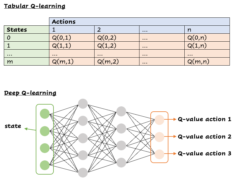
Q-learning is a reinforcement learning algorithm where an agent learns to maximize rewards through interactions with the environment. It uses a Q-function Q(s, a) to predict future rewards. The agent updates the Q-values using the Bellman equation, adjusting its predictions based on the received rewards and the expected future rewards.

Practical Example

Imagine being in state sss with a predicted Q(s, a) = 100. After taking action a, you transition to state s' and receive a reward of 8. The Q-value for the best action in s' is 95, with a discount factor of 0.99. The temporal difference is ${{8 + 0.99 \times 95 - 100 = 2.05}}$. With a learning rate of 0.1, the updated Q-value becomes ${{100 + 0.1 \times 2.05 = 100.205}}$.

Deep Q-Learning

Traditional Q-learning uses a table to store Q-values, which is infeasible for environments with many states and actions. DQN uses a neural network to approximate Q(s, a), allowing the agent to generalize to unseen state-action pairs. The input to the neural network is an observation, and the output is a Q-value for each possible action.

DQN Algorithm

Experience Replay: Stores experiences (s, a, r, s') in a replay buffer. Random sampling from the buffer helps break temporal correlations, making learning more stable.
Target Network: Uses two neural networks: the primary network for decision-making and the target network for providing stable Q-value targets.
Training Steps:

Initialize replay buffer and networks.

For each episode:

Initialize starting state.

For each step:

Select action aaa using an ϵ\epsilonϵ-greedy policy.
Execute action and observe reward r and next state s'.
Store experience in replay buffer.
Sample mini-batch from replay buffer.
Compute target Q-value and perform gradient descent on the loss.
Update target network periodically.

Enhancements for Stability

To ensure stability and convergence, several enhancements are implemented:

E-greedy Action Selection: Balances exploration and exploitation by adjusting the exploration rate over time.
Experience Replay: Allows learning from batches of past experiences, ensuring stable training and better convergence.
Target vs. Local Network: Uses a target network to provide stable Q-value targets, reducing oscillations and divergence.

Target vs. Local Network

In DQN, two networks are used to stabilize learning:

Primary (Local) Network: This network is updated continuously and is used to select actions during training. It learns by minimizing the loss between predicted Q-values and target Q-values.
Target Network: This network provides stable targets for the Q-value updates. Unlike the primary network, the target network's weights are updated less frequently, typically by copying the primary network's weights every few thousand steps.

Why Use Two Networks?

Stability: The primary network's weights are updated frequently, which can lead to instability and divergence. By using the target network to provide stable Q-value targets, we avoid rapid oscillations in learning.
Consistency: The target network helps maintain consistent learning targets, as it is only updated periodically. This ensures that the Q-value updates are based on more stable and reliable targets, leading to smoother and more stable learning.

Update Mechanism

Primary Network Update: After each action, the primary network updates its weights using the loss computed from the difference between the predicted Q-values and the target Q-values provided by the target network.
Target Network Update: Every few thousand steps, the weights of the primary network are copied to the target network, ensuring that the target network provides stable targets for a certain number of steps before being updated again.

‍

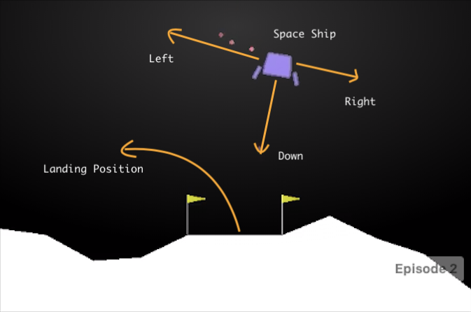
Here is a detailed code example:

Step 1: Install Required Libraries

1pip install gymnasium gymnasium[box2d] stable-baselines3 torch

Step 2: Import Libraries and Setup Environment

1import gym
2from stable_baselines3 import DQN
3from stable_baselines3.common.evaluation 
4import evaluate_policy
5
6# Create the Lunar Lander environment
7env = gym.make("LunarLander-v2")

Step 3: Define the DQN Model

1# Define the DQN model
2model = DQN("MlpPolicy", env, verbose=1)

Step 4: Train the DQN Model

1# Train the model
2model.learn(total_timesteps=100000)  # Adjust the timesteps as needed

Step 5: Evaluate the Trained Model

1# Evaluate the trained mode
2lmean_reward, std_reward = evaluate_policy(model, env, n_eval_episodes=10)
3print(f"Mean reward: {mean_reward} +/- {std_reward}")
4
5# Optionally, save the model
6model.save("dqn_lunar_lander")

Step 6: Visualize the Trained Model

1import time
2# Load the model if needed
3# model = DQN.load("dqn_lunar_lander")
4# Visualize the model's performanceepisodes = 5
5
6for episode in range(1, episodes + 1):    
7	obs = env.reset()    
8    done = False    
9    score = 0    
10    while not done:        
11    	env.render()        
12        action, _states = model.predict(obs)        
13        obs, reward, done, info = env.step(action)        
14        score += reward    
15    print(f"Episode: {episode}, Score: {score}")    
16	time.sleep(1)
17env.close()

Explanation

Environment Setup: `gym.make("LunarLander-v2")` initializes the Lunar Lander environment.
DQN Model: The `DQN` class from Stable Baselines3 is used to define the model with an MLP policy.
Training: The `learn` method trains the model with the specified number of time-steps.
Evaluation: The `evaluate_policy` function assesses the model's performance over several episodes.
Visualization: The loop renders the environment to visualize how the trained model performs in real-time.

Additional Tips

Hyper-parameters: You might need to tune the hyper-parameters (like learning rate, batch size, etc.) for better performance.
Checkpointing: Save intermediate models during training to prevent loss of progress.
Monitoring: Use TensorBoard for monitoring training metrics in real-time.

‍

‍

Conclusion

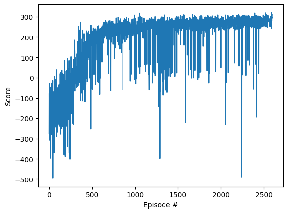
DQN is a powerful reinforcement learning algorithm combining Q-learning and deep neural networks. By utilizing techniques such as experience replay and target networks, DQN effectively learns to solve complex environments like Gymnasium's Lunar Lander, demonstrating its potential in both gaming and real-world applications. The use of a target network alongside the primary network ensures stability and consistency in learning, making DQN a robust and efficient algorithm for a wide range of RL problems.

Cost and Execution Time

This was trained using the Google Colab Pro GPU T4

Additional Learning Materials

Code Repository & Models

Updated On:

December 10, 2024

Follow on social media: