Comparing how PPO, SAC, and DQN Perform on Gymnasium's Lunar Lander

Introduction

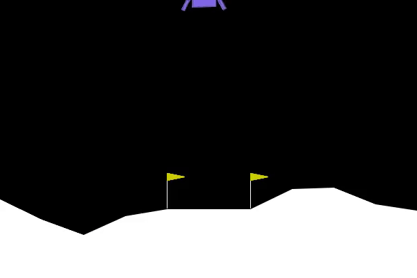
The Lunar Lander environment, a popular benchmark in OpenAI's Gym, challenges an agent to land a spacecraft safely on a designated landing pad. The environment provides continuous state and action spaces, making it a suitable candidate for testing different reinforcement learning (RL) algorithms. This blog post explores how three advanced RL algorithms—Proximal Policy Optimization (PPO), Soft Actor-Critic (SAC), and Deep Q-Network (DQN)—can be used to solve the Lunar Lander problem.

Understanding the Algorithms

Proximal Policy Optimization (PPO)

PPO is an on-policy algorithm that balances simplicity and performance. Here's how PPO learns:

Policy Optimization: PPO uses a stochastic policy, which means it outputs a probability distribution over actions rather than a single deterministic action. The policy is optimized using a surrogate objective function.
Clipping Mechanism: To prevent large updates that could destabilize training, PPO introduces a clipping mechanism. The probability ratio between the new and old policies is clipped to ensure the policy does not change too drastically between updates.
Advantages Estimation: PPO relies on advantage estimation, which is the difference between the expected return (value function) and the actual return. This helps the algorithm focus on actions that are better than average.
Epochs and Batching: The algorithm updates the policy by iterating over multiple epochs and mini-batches, which ensures efficient and stable learning.

Stochastic Policy in PPO

A stochastic policy in PPO outputs a probability distribution over actions. This allows the agent to sample different actions even in the same state, promoting exploration and reducing the chance of getting stuck in local optima. The stochastic policy is typically modeled using a Gaussian distribution for continuous action spaces, where the mean and standard deviation are learned parameters.

The advantage of using a stochastic policy is that it encourages the agent to explore the environment more thoroughly, which can lead to discovering better strategies that deterministic policies might miss. The exploration-exploitation trade-off is crucial in RL, and a stochastic policy provides a natural way to balance this trade-off.

The Role of Entropy in Encouraging Exploration in PPO

Balancing exploration and exploitation is vital in reinforcement learning, and PPO addresses this challenge through entropy.

What is Entropy?

In this context, entropy measures the randomness or uncertainty in the action distribution of the policy. High entropy indicates more random action selection, while low entropy suggests a more deterministic approach.

How Entropy Encourages Exploration

Entropy is integrated into PPO by adding an entropy bonus to the loss function. This bonus encourages the policy to maintain a level of randomness during training, preventing premature convergence to suboptimal policies. Essentially, the entropy term helps the agent to keep exploring different actions, leading to a more comprehensive understanding of the environment.

The entropy term in the loss function typically takes the form:

$${{\text{Loss} = \text{Policy Loss} - \lambda \times \text{Entropy}}}$$

Here, ${{\lambda}}$ is a hyper-parameter that controls the weight of the entropy bonus. A higher value of λ\lambdaλ leads to more exploration, while a lower value favors exploitation.

Balancing Exploration and Exploitation

The right balance between exploration and exploitation is essential for effective learning. Too much exploration can delay convergence by spending too much time on suboptimal actions, while too little exploration can cause the policy to converge prematurely to a local minimum. PPO manages this balance by gradually reducing the entropy bonus as training progresses, allowing the algorithm to focus more on exploitation once sufficient knowledge about the environment has been gathered.

Practical Considerations

When tuning the entropy coefficient λ\lambdaλ, consider the specific problem and environment. Higher entropy might be beneficial in environments with high variability or complex dynamics, while a lower entropy bonus might suffice in more straightforward environments.

By managing entropy effectively, PPO ensures that the agent explores sufficiently before committing to a strategy, leading to more robust and generalizable policies.

Soft Actor-Critic (SAC)

SAC is an off-policy algorithm designed for continuous action spaces. Here's how SAC learns:

Actor-Critic Framework: SAC employs an actor (policy) and two critics (value functions). The actor selects actions, while the critics evaluate them.
Entropy Regularization: SAC maximizes both the expected return and the entropy of the policy. Entropy regularization encourages exploration by adding a term to the objective function that measures the randomness of the policy. This helps prevent premature convergence to suboptimal policies.
Off-Policy Learning: SAC leverages a replay buffer to store and reuse past experiences, which improves sample efficiency. The critics are updated using batches of experiences drawn from the replay buffer.
Soft Q-Learning: SAC uses a soft version of the Bellman equation to update the critics. This involves minimizing the difference between the predicted Q-values and the target Q-values, which include the entropy term.

Entropy Regularization in SAC

Entropy regularization in SAC introduces an entropy term to the objective function, which encourages the policy to maintain randomness. The entropy term ${{H(\pi(\cdot|s))}}$ is added to the reward, where ${{\pi}}$ is the policy and sss is the state. This term penalizes certainty in action selection, incentivizing the agent to explore different actions rather than sticking to a deterministic policy.

The objective function in SAC becomes: ${{J(\pi) = \sum_{t=0}^{T} \mathbb{E}_{(s_t, a_t) \sim \rho_\pi} \left[ r(s_t, a_t) + \alpha H(\pi(\cdot|s_t)) \right]}}$ where ${{alpha}}$ is a temperature parameter that controls the trade-off between reward maximization and entropy maximization.

By encouraging higher entropy, the agent is more likely to explore diverse actions, which can lead to discovering better long-term strategies. This makes SAC particularly effective in environments where exploration is crucial for finding optimal policies.

Actor-Critic Framework in SAC

In SAC, the actor-critic framework is fundamental to its learning process. The framework consists of two main components:

Actor (Policy Network): The actor is responsible for selecting actions based on the current state. It outputs a probability distribution over actions (a stochastic policy), which ensures diverse action selection and promotes exploration. The policy network is trained to maximize the expected return and the entropy of the policy, balancing exploitation and exploration.
Critics (Q-Value Networks): SAC employs two Q-value networks (critics) to estimate the expected return of taking an action in a given state. Having two critics helps in reducing overestimation bias, which is common in Q-learning algorithms. The critics are trained to minimize the Bellman error, ensuring accurate value estimation.

The learning process involves alternating updates between the actor and the critics:

Critic Update: The critics are updated using the soft Bellman equation. The target Q-value is computed considering both the reward and the entropy term, which encourages the policy to remain stochastic.
Actor Update: The actor is updated by maximizing the expected return and the entropy of the policy. The policy gradient is computed using the critics' Q-values, guiding the actor towards actions that yield higher returns while maintaining exploration.

This interplay between the actor and critics allows SAC to effectively learn policies that balance exploration and exploitation, making it a powerful algorithm for continuous action spaces.

Deep Q-Network (DQN)

DQN is an off-policy algorithm typically used for discrete action spaces. For the Lunar Lander environment, we adapt it to handle continuous state spaces. Here's how DQN learns:

Q-Value Approximation: DQN uses a neural network to approximate the Q-value function, which estimates the expected return of taking a certain action in a given state.
Experience Replay: DQN stores past experiences in a replay buffer and samples mini-batches of experiences during training. This breaks the correlation between consecutive experiences and improves learning stability.
Target Networks: DQN employs a target network to stabilize training. The target network is a copy of the Q-network and is updated less frequently. This reduces the likelihood of divergence during training.
Epsilon-Greedy Policy: DQN uses an epsilon-greedy policy to balance exploration and exploitation. With probability epsilon, the agent selects a random action; otherwise, it selects the action with the highest Q-value.

Continuous vs. Discrete Action Spaces

The choice between continuous and discrete action spaces significantly impacts the design and performance of RL algorithms.

Continuous Action Spaces

Continuous action spaces provide a range of possible actions, making them suitable for tasks requiring fine control, such as robotic manipulation or the Lunar Lander environment. Algorithms designed for continuous action spaces, like PPO and SAC, must handle a continuous range of values for each action dimension.

PPO: Uses a stochastic policy, typically modeled by a Gaussian distribution, to output continuous actions. This allows PPO to handle the fine-grained control needed in continuous action environments effectively.
SAC: Also employs a stochastic policy with a Gaussian distribution, but it enhances exploration through entropy regularization. The continuous action space allows SAC to leverage the entropy term to maintain diverse action selection, preventing premature convergence.

Discrete Action Spaces

Discrete action spaces consist of a finite set of actions, making them suitable for tasks with clear, distinct actions, such as playing video games or board games. DQN is designed for discrete action spaces and operates by selecting the action with the highest Q-value.

DQN: Uses a neural network to approximate the Q-values for each discrete action. The agent selects actions using an epsilon-greedy policy, balancing exploration and exploitation. While DQN can be adapted for continuous state spaces, its original design is tailored to discrete actions.

Implementing the Algorithms

Let's dive into the implementation of each algorithm for the Lunar Lander environment.

1. Proximal Policy Optimization (PPO)

1import gymnanisum as gym
2from stable_baselines3 import PPO
3
4# Create the Lunar Lander environment
5env = gym.make("LunarLander-v2")
6
7# Initialize the PPO model
8model = PPO("MlpPolicy", env, verbose=1)
9
10# Train the model
11model.learn(total_timesteps=100000)
12
13# Save the model
14model.save("ppo_lunar_lander")
15
16# Evaluate the model
17obs = env.reset()
18for _ in range(1000):    
19	action, _states = model.predict(obs)    
20    obs, rewards, dones, info = env.step(action)    
21    env.render()
22env.close()

2. Soft Actor-Critic (SAC)

1import gymnasium as gym
2from stable_baselines3 import SAC
3
4# Create the Lunar Lander environment
5env = gym.make("LunarLanderContinuous-v2")
6
7# Initialize the SAC model
8model = SAC("MlpPolicy", env, verbose=1)
9
10# Train the model
11model.learn(total_timesteps=100000)
12
13# Save the model
14model.save("sac_lunar_lander")
15
16# Evaluate the mode
17lobs = env.reset()
18for _ in range(1000):    
19	action, _states = model.predict(obs)
20    obs, rewards, dones, info = env.step(action)
21    env.render()
22env.close()

3. Deep Q-Network (DQN)

1import gymnasium as gym
2from stable_baselines3 import DQN
3
4# Create the Lunar Lander environment
5env = gym.make("LunarLander-v2")
6
7# Initialize the DQN model
8model = DQN("MlpPolicy", env, verbose=1)
9
10# Train the model
11model.learn(total_timesteps=100000)
12
13# Save the model
14model.save("dqn_lunar_lander")
15
16# Evaluate the model
17obs = env.reset()
18for _ in range(1000):
19	action, _states = model.predict(obs)
20    obs, rewards, dones, info = env.step(action)
21    env.render()
22env.close()

‍

Comparison and Results

Each of these algorithms has its strengths and weaknesses when applied to the Lunar Lander environment:

PPO: Provides a good balance between exploration and exploitation, making it suitable for environments with continuous state and action spaces. It usually converges faster and is more stable.
SAC: Offers robust exploration through entropy regularization, often leading to better performance in environments with continuous action spaces. However, it may require more computational resources and longer training times.
DQN: While traditionally used for discrete action spaces, it can be adapted for the Lunar Lander environment. It generally performs well but may not be as effective as PPO or SAC for continuous action spaces.

Conclusion

Solving the Lunar Lander environment using PPO, SAC, and DQN showcases the versatility and strengths of these advanced RL algorithms. By leveraging the unique properties of each algorithm, we can achieve efficient and effective solutions to this challenging problem. Whether you prioritize stability, exploration, or computational efficiency, there is an RL algorithm well-suited for your needs.

Additional Learning Materials

Code Repository & Models

Follow on social media: